AI building blocks - from scratch with Python
Linear regression and gradient descent are techniques that form the basis of many other, more complicated, ML/AI techniques (e.g., deep learning models). They are, thus, building blocks that all ML/AI engineers need to understand.
Regression
Regression is a process in which we model how one variable (for example, sales) changes with respect to another variable (for example, number of users). Generally, regression techniques in machine learning are concerned with predicting continuous values (for example, stock price, temperature, or disease progression). Classification, on the other hand, is concerned with predicting discrete variables, or one of a discrete set of categories (for example, fraud/not fraud, sitting/standing/running, or hot dog/not hot dog).
Linear regression, as you might expect, models the relationship a response (e.g., sales) and a feature (e.g., users) using the equation for a line:
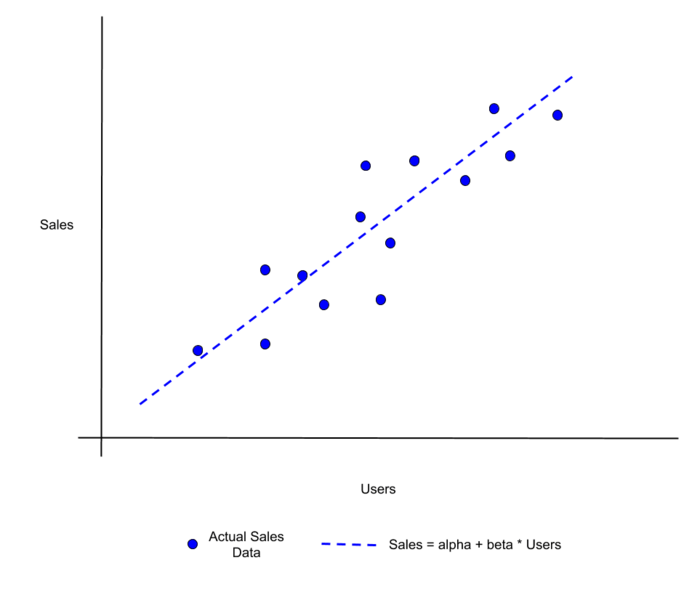
The parameters, alpha and beta, represent:
alpha - the intercept (or bias) of the line (i.e., where the line crosses the y axis in the above plot)
beta - the slope (or weight) of the line (i.e., how quickly the value of sales changes up or down as the value of users changes)
Remember, an ML model is simply a certain kind of parameterized function. You put data in and the function transforms that data into a prediction via one more parameters. In this case, the linear regression model take a numerical feature in and uses the intercept and slope parameters to transform that numerical feature into another number, which number is a prediction of our response.
“Training” this linear regression model is, thus, the process of figuring out the particular intercept and slope that fits our line as close as possible to our data examples. In the above example, we would want the particular intercept and slope that allows us to predict sales as close as possible, as evaluated on actual sales data points. But how do we find the ideal intercept and slope?
The answer: we choose the parameters that get our line “closest” to all of the known data points. To do that, we need a way to measure the error (or loss) between the known data points (what we should be predicting with our model) and the predictions produced by our formula for the line. One choice for this error/loss is the squared error defined as follows with a Python function:
def squared_error(prediction, observation):
    """
    Calculates the squared error.

    Args:
        prediction - the prediction from our LR model
        observation - the observed data point
    Returns:
        The squared error
    """
    return (observation - prediction) ** 2
We then need to minimize this, and, as it turns out, this minimization has an exact mathematical solution. It’s called the ordinary least square (OLS) solution and here is an implementation:
def ols_fit(x, y):
    """
    Calculates the intercept/slope using OLS.

    Args:
        x - feature array
        y - response array
    Returns:
        The intercept and slope parameters
    """

    # calculate the mean of x and y
    mean_x = np.mean(x)
    mean_y = np.mean(y)

    # Using the derived OLS formula to calculate
    # the intercept and slope.
    numerator = 0
    denominator = 0
    for i in range(len(x)):
        numerator += (x[i] - mean_x) * (y[i] - mean_y)
        denominator += (x[i] - mean_x) ** 2
    slope = numerator / denominator
    intercept= mean_y - (slope * mean_x)

    return intercept, slope
Gradient descent
As mentioned above, an exact mathematical solution for our intercept and slope exists using OLS, so why use anything else? Well, it turns out that the OLS solution is pretty fast and simple for the single regression case we are considering here (i.e., when we are modeling our response by changes in a single feature). Once we move into more complicated cases, however, we are going to want to model our response by changes in multiple other features (e.g., with what’s called “multiple regression”). In those cases, the exact solution is more complicated and much less computationally efficient.
Enter gradient descent. Gradient descent is an iterative method that starts with some initial choice of intercept and slope and then iteratively makes adjustments to the intercept and slope until an error/loss is minimized. Basically, it just tries a bunch of choices for our model line until it minimizes the error.
Note - Exactly how those adjustments to the intercept and slope take place on each iteration differs in different flavors of gradient descent, which include batch gradient descent, stochastic gradient descent, mini-batch gradient descent. You can learn more about these flavors here. We will focus on “stochastic” gradient descent here for illustrative purposes (and because it is so widely used).
The iterative process goes like this for the “stochastic” version of gradient descent (SGD):
Initialize our intercept and slope (e.g., via a random seed or by setting them to zero)
For each iteration (or epoch):
Using a current value for the intercept and slope, calculate predictions for all the feature and response points in the data set
Calculate the error between those predictions and the observed response values using a definition for error/loss
Calculate a “gradient” value for the slope and intercept based on our definition for error/loss (more details below)
Update the intercept and slope according to the gradient values
Sometimes the loop represented above in step (2) is repeated for a fixed number of epochs (as we will do in our example). In other implementations, the loop might continue until the error isn’t changing between iterations (within a certain tolerance) or until it hits a maximum number of iterations.
The gradient values mentioned above are based on the derivatives of the function that we are using to calculate our error/loss (sometimes called a cost function). If you aren’t familiar with derivatives, this basically means that we are using a function that can tell us the direction of the greatest rate of increase/decrease of another function. We want to minimize our error, so we want to change our intercept and slope parameters in a “direction” that moves to lower error. That’s why we calculate a gradient value for each of the slope and intercept (to find that direction) and use those gradient values to update the intercept and slope.
Here is an implementation in Python to make things more concrete:
def sgd_fit(x, y, learning_rate, epochs):
    """
    Calculates the intercept/slope using SGD.

    Args:
        x - feature array
        y - response array
        learning_rate - learning rate
        epochs - the number of epochs for the SGD loop
    Returns:
        intercept, slope and error
    """

    # initialize the slope and intercept
    slope = 0.0
    intercept = 0.0

    # set the number of observations in the data
    N = float(len(y))

    # loop over the number of epochs
    for i in range(epochs):

        # calculate our current predictions
        predictions = (slope * x) + intercept

        # calculate the sum of squared errors
        error = sum([data**2 for data in (y-predictions)]) / N

        # calculate the gradients for the slope and intercept
        slope_gradient = -(2/N) * sum(x * (y - predictions))
        intercept_gradient = -(2/N) * sum(y - predictions)

        # update the slope and intercept
        slope = slope - (learning_rate * slope_gradient)
        intercept = intercept - (learning_rate * intercept_gradient)

    return intercept, slope, error
In most gradient descent algorithms, the update of the parameters involves multiplying our gradients by a learning rate, rather than just using the raw gradient values. This learning rate is an additional parameter that can be tweaked to improve model training/convergence (also known as a hyperparameter). By setting the learning rate smaller, you will be making the updates to the intercept and slope less dramatic (i.e., smaller), and, in this way, you can avoid numerical oscillations during convergence, which might prevent you from minimizing error. However, this will also cause the algorithm to converge slower. You often need to experiment with the learning rate a bit so as to find an appropriate balance between well-behaved convergence and computational efficiency.
Note - here we are just trying to find two ideal parameters (a slope, or weight, and an intercept, or bias). In more complicated models (like neural networks) we might be trying to find thousands of ideal weights and biases. That’s where algorithms like SGD are essential in the training process.
Third-party packages for OLS and SGD
Even though we use the above pattern of SGD minimization throughout ML/AI methods, we don’t have to implement it (or OLS) from scratch every time. As you might expect, there are some great implementations of OLS and SGD in existing Python packages. Below are some examples ways of determining our intercept and slope with the statsmodels, scikit-learn, and PyTorch packages.
OLS with statsmodels:
def sm_ols_fit(x, y):
    """
    Calculates the intercept/slope using OLS.

    Args:
        x - feature array
        y - response array
    Returns:
        The intercept and slope parameters
    """

    # add a constant column to the x values which
    # represents the intercept
    x = sm.add_constant(x)

    # define the OLS model
    model = sm.OLS(y, x)

    # train the model
    results = model.fit()

    return results.params[0], results.params[1]
OLS with scikit-learn:
def sklearn_ols_fit(x, y):
    """
    Calculates the intercept/slope using OLS.

    Args:
        x - feature array
        y - response array
    Returns:
        The intercept and slope parameters
    """

    # define the model
    lr = linear_model.LinearRegression()

    # train the model
    lr.fit(x[:, np.newaxis], y)

    return lr.intercept_, lr.coef_[0]
SGD with scikit-learn:
def sklearn_sgd_fit(x, y):
    """
    Calculates the intercept/slope using SGD.

    Args:
        x - feature array
        y - response array
    Returns:
        The intercept and slope parameters
    """

    # define the model
    lr = linear_model.SGDRegressor(max_iter=1000)

    # traing the model
    lr.fit(x[:, np.newaxis], y)

    return lr.intercept_[0], lr.coef_[0]
SGD with PyTorch:
class PyTorchLRModel(torch.nn.Module):

    def __init__(self, input_dim, output_dim):

        # call class constructor
        super(PyTorchLRModel, self).__init__()

        # use the nn package to create a linear layer
        self.linear = torch.nn.Linear(input_dim, output_dim)

    def forward(self, x):

        # Define the "forward" pass of this model. Think of this
        # for now as just the method that takes data input and
        # passes this through the model to create output.
        out = self.linear(x)
        return out

def pytorch_sgd_fit(x, y, learning_rate, epochs):
    """
    Calculates the intercept/slope using SGD.

    Args:
        x - feature array
        y - response array
        learning_rate - learning rate used in SGD
        epochs - number of epochs for the SGD loop
    Returns:
        The intercept and slope parameters
    """

    # create the model using only one "node", which will
    # correspond to our single linear regression model
    input_dimension = 1
    output_dimension = 1

    # define the model
    model = PyTorchLRModel(input_dimension, output_dimension)

    # our error/loss function
    criterion = torch.nn.MSELoss()

    # define our SGD optimizer
    optimiser = torch.optim.SGD(model.parameters(), lr = learning_rate)

    # loop over our epochs, similar to our previous implementation
    for epoch in range(epochs):

        # increment the epoch count
        epoch +=1

        # define our feature and response variables
        features = Variable(torch.from_numpy(x[:, np.newaxis]).float())
        response = Variable(torch.from_numpy(y[:, np.newaxis]).float())

        #clear the gradients
        optimiser.zero_grad()

        # calculate the predicted values
        predictions = model.forward(features)

        # calculate our loss
        loss = criterion(predictions, response)

        # implement our gradient-based updates to our
        # parammeters (putting them "back" into the model
        # via a "backward" update)
        loss.backward()
        optimiser.step()

    # extract the model parameters to return
    params = []
    for param in model.parameters():
        params.append(param.data[0])

    return params[1].item(), params[0][0].item()
Note - The PyTorch example is unique in that it closely mimics the structure of our from-scratch SGD example. However, if you look closely, you will see some useful pytorch functionality that allowed us to easily define our cost function and update our intercept and slope. These built-in functions allow us to efficiently train much more complicated models on specialized architectures (like GPUs), while keeping our SGD optimization loop relatively simple.
Note - The PyTorch example is also unique in that it shows how we can define our own model class for training, whereas the other example utilized more “black-box” or “pre-baked” approaches.
Example
Let’s make these example concrete with an example. Imagine that we are wanting to model our company’s sales based on our advertising spend. Our data might look something like (full data set here):
TV,Radio,Newspaper,Sales
230.1,37.8,69.2,22.1
44.5,39.3,45.1,10.4
17.2,45.9,69.3,9.3
151.5,41.3,58.5,18.5
180.8,10.8,58.4,12.9
8.7,48.9,75,7.2
57.5,32.8,23.5,11.8
120.2,19.6,11.6,13.2
8.6,2.1,1,4.8
In particular, we might be interested in predicting our sales (last column) based on our TV advertising spend (represented by the first column). Using linear regression, we could try to model this as:
Sales = alpha + beta * TV
To find alpha (the intercept) and beta (the slope) we could use our model fitting functions defined above. However, before providing our data to those functions we should take care of one issue in pre-processing.
You will notice that the values of TV are, at least in some cases, an order of magnitude larger than our Sales values. This difference in scaling could create numerical inefficiencies for our iterative SGD algorithms as it try to make it parameter updates. Even worse, it could prevent our optimization from converging, or it could artificially emphasize one feature over another (if we were using multiple features in our model).
Thankfully, scikit-learn provides us with a convenient way to scale the values of each of these variables between 0 and 1. Here is the implementation along with the utilization of our fitting functions:
def main():

    # import the data
    data = pd.read_csv('../data/Advertising.csv')

    # scale the feature and response
    scaler = MinMaxScaler()
    data_scaled = scaler.fit_transform(data[['TV', 'Sales']])

    # fit our model using our various implementations
    int_ols, slope_ols = ols_fit(data_scaled[:, 0], data_scaled[:, 1])
    int_sgd, slope_sgd, _ = sgd_fit(data_scaled[:, 0], data_scaled[:, 1], 0.1, 1000)
    int_sm_ols, slope_sm_ols = sm_ols_fit(data_scaled[:, 0], data_scaled[:, 1])
    int_sk_ols, slope_sk_ols = sklearn_ols_fit(data_scaled[:, 0], data_scaled[:, 1])
    int_sk_sgd, slope_sk_sgd = sklearn_sgd_fit(data_scaled[:, 0], data_scaled[:, 1])
    int_pt_sgd, slope_pt_sgd = pytorch_sgd_fit(data_scaled[:, 0], data_scaled[:, 1], 0.1, 1000)

    # output the results
    delim = "-----------------------------------------------------------------"
    print("\nOLS\n{delim}\n intercept: {intercept}, slope: {slope}"
            .format(delim=delim, intercept=int_ols, slope=slope_ols))
    print("\nSGD\n{delim}\n intercept: {intercept}, slope: {slope}"
            .format(delim=delim, intercept=int_sgd, slope=slope_sgd))
    print("\nstatsmodels OLS\n{delim}\n intercept: {intercept}, slope: {slope}"
            .format(delim=delim, intercept=int_sm_ols, slope=slope_sm_ols))
    print("\nsklearn OLS\n{delim}\n intercept: {intercept}, slope: {slope}"
            .format(delim=delim, intercept=int_sk_ols, slope=slope_sk_ols))
    print("\nsklearn SGD\n{delim}\n intercept: {intercept}, slope: {slope}"
            .format(delim=delim, intercept=int_sk_sgd, slope=slope_sk_sgd))
    print("\npytorch SGD\n{delim}\n intercept: {intercept}, slope: {slope}"
            .format(delim=delim, intercept=int_pt_sgd, slope=slope_pt_sgd))

if __name__ == "__main__":
    main()
This outputs:
$ python3 main.py
/usr/local/lib/python3.7/site-packages/sklearn/linear_model/base.py:509: RuntimeWarning: internal gelsd driver lwork query error, required iwork dimension not returned. This is likely the result of LAPACK bug 0038, fixed in LAPACK 3.2.2 (released July 21, 2010). Falling back to 'gelss' driver.
  linalg.lstsq(X, y)

OLS
-----------------------------------------------------------------
 intercept: 0.21519170068625232, slope: 0.5534088415765329

SGD
-----------------------------------------------------------------
 intercept: 0.21519198226718594, slope: 0.5534083104180343

statsmodels OLS
-----------------------------------------------------------------
 intercept: 0.21519170068625226, slope: 0.5534088415765327

sklearn OLS
-----------------------------------------------------------------
 intercept: 0.21519170068625243, slope: 0.5534088415765327

sklearn SGD
-----------------------------------------------------------------
 intercept: 0.21555094152403473, slope: 0.5526580223168277

pytorch SGD
-----------------------------------------------------------------
 intercept: 0.21519266068935394, slope: 0.5534069538116455
This shows how the different methods produce very similar results, and it shows that there isn’t any magic under the hood of these ML packages. They are just implementing a series of well-understood and concretely defined methods.
Finally, let’s plot the line that we have fit to our data alongside the actual data that we used to fit the line. This will give us a visual indication of how the model is tracking with actual observations.
import numpy as np
import pandas as pd
import matplotlib.pyplot as plt
from sklearn.preprocessing import MinMaxScaler

# import the data
data = pd.read_csv('../data/Advertising.csv')

# scale the feature and response
scaler = MinMaxScaler()
data_scaled = scaler.fit_transform(data[['TV', 'Sales']])
data_scaled_df = pd.DataFrame(data_scaled, columns=['TV', 'Sales'])

# calculate modeled values for Sales based on our
# linear regression model
slope = 0.553
intercept = 0.215
data_scaled_df['Model'] = data_scaled_df['TV'].apply(lambda x: slope * x + intercept)

# create the plot
fig, ax = plt.subplots()
ax.plot(data_scaled_df['TV'].values, data_scaled_df['Model'].values, 'k--')
ax.plot(data_scaled_df['TV'].values, data_scaled_df['Sales'].values, 'ro')
plt.xlabel('TV', axes=ax)
plt.ylabel('Sales', axes=ax)

# Only draw spine between the y-ticks
ax.spines['left'].set_bounds(0, 1)

# Hide the right and top spines
ax.spines['right'].set_visible(False)
ax.spines['top'].set_visible(False)

# Only show ticks on the left and bottom spines
ax.yaxis.set_ticks_position('left')
ax.xaxis.set_ticks_position('bottom')

plt.show()
This will create the following plot:

where the red dots represent actual Sales data and the dashed line is our linear regression model.
If you have even more interest in leveling up your AI skills (maybe you want to transition from software engineer to AI practicioner), consider joining us for the AI Classroom event. AI Classroom is an immersive, 3 day virtual training event for anyone with at least some programming experience and foundational understanding of mathematics. The training provides a practical baseline for realistic AI development using Python and open source frameworks like TensorFlow and PyTorch. After completing the course, participants will have the confidence to start developing and deploying their own AI solutions.